
“Order and simplification are the first steps toward mastery of a subject — the actual enemy is the unknown.”
Thomas Mann
As a new SQL developer, do you remember being frustrated that you couldn’t use the alias of a COUNT(*) in the predicate/WHERE clause, but you could in the ORDER BY? Or have you been confused on when you should put something in the ON clause vs the WHERE clause vs the HAVING clause? This article will help clear that all up and it all has to do with how SQL Server processes your query.
Why SQL Isn’t Like Other Languages
Most developers are used to writing code top to bottom and expecting the computer to execute that code in the same order. However, unlike those procedural languages, SQL is a declarative language. In a procedural language, you give the computer specific set of directions telling it how to do tasks. In a declarative language, you give the computer what you want it to return and it determines how it will do that (using the Query Optimizer). This often confuses first time SQL developers; especially when they believe SQL Server is doing all the tasks from the top down in the query. In fact, it may even surprise many seasoned SQL Developers to learn that SQL Server actually starts in the middle of your query.
*Many thanks to Itzik Ben-Gan and his books for helping solidify this in my brain several years ago! I highly recommend reading them if you want to go even deeper into this.*
TL;DR:
The T-SQL Logical Processing Order:
- FROM
- JOIN
- ON
- WHERE
- GROUP BY
- HAVING
- SELECT
- DISTINCT
- ORDER BY
- TOP
Lets take this query as an example for our discussion:
SELECT TOP 50 e.EmployeeName Name, DATEDIFF(Year, e.StartDate, GETDATE()) YearsEmployed, SUM(s.SalesAmt) Total_SalesAmt
FROM dbo.EmpTable e
LEFT JOIN dbo.SalesTable s
ON e.EmpID = S.EmpID
AND s.Type = 'Software'
WHERE e.Region = 'North'
GROUP BY e.EmployeeName, DATEDIFF(Year, e.StartDate, GETDATE())
HAVING SUM(s.SalesAmt) >= 1000
ORDER BY YearsEmployed DESC, SUM(s.SalesAmt) DESC, e.EmployeeName
Most people who write SQL write it from the top down starting with SELECT (maybe leaving that with a * until you decide what fields you want to put in there), moving on to FROM, the JOIN(s), a WHERE clause, a GROUP BY, the HAVING, and finally the ORDER BY.
The Logical Order vs. The Written Order
However, SQL Server actually reads/processes the query in this logical order: FROM, JOIN(s), ON, WHERE, GROUP BY, HAVING, SELECT, DISTINCT, ORDER BY, and finally TOP.
It is important to note here we are talking about the Logical processing order. This is how SQL Server is going to read your query to make sense of it. It will then pass this information on over to have a query plan created which will be the Physical processing order, which is how it will actually gather the data from the tables and return the results.
A Step-by-Step Walkthrough of Query Processing
SQL Server starts with the raw tables themselves , and filters down the rows before it gets to the specific columns you want returned. This can have a significant impact on how and what you can put in your different sections of the query.
Phase 1: FROM – Gathering the Raw Data
In the first phase, SQL Server pulls back all records and all rows from the table after the FROM clause. Note: It does not limit to any specific rows (because at this point it does not know any predicate information) nor does it limit to any specific columns (because at this point it does not know any columns you want returned in your SELECT clause).
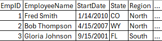
(1) FROM dbo.EmpTable e
Below you see what we’ll call ResultSet1 from Phase 1 (the … represents all the other fields in this table, you’ll see the same for the next several phases). The FROM clause is one of two mandatory clause that every query must have.
Phase 2 & 3: JOIN and ON – Combining and Filtering Tables
The second phase does your join(s). At this point SQL Server does a cartesian join between ResultSet1 from above to your tables in the join (in this case the dbo.SalesTable). This is a cartesian join (every row from ResultSet1 is matched to every row from your table), because SQL Server has not read any of the ON criteria yet.
As a side note: This phase also includes APPLY, PIVOT, and UNPIVOT.
(1) FROM dbo.EmpTable e
(2) LEFT JOIN dbo.SalesTable s
Lets say below is the first few rows of the dbo.SalesTable:
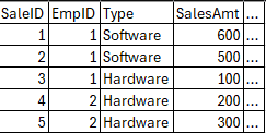
Below is what the ResultSet2 would look like after Phase 2 with the cartesian join:
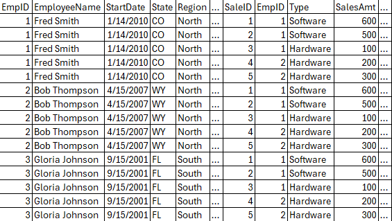
Next in Phase 3, we would apply the ON clause of the join. This would filter our cartesian join based on whatever criteria we may have in this clause.
(1) FROM dbo.EmpTable e
(2) LEFT JOIN dbo.SalesTable s
(3) ON e.EmpID = S.EmpID
AND s.Type = ‘Software’
In our example, this will remove the “extra joins” of the cartesian join (where the EmpIDs don’t match). It will also only keep rows where the type is Software. As you can see below, this means we have both SalesTable rows for Fred since they are Software, but then for Bob and Gloria we see nothing from SalesTable. But we do still see their data from the EmpTable since we have a LEFT JOIN.

At this point, SQL Server would repeat Phases 2 and 3 for each table you are joining on. In our example, though, we have no more tables.
Phase 4: WHERE – Applying the First Filters
Now we move on to Phase 4 which is the WHERE criteria. This is where many developers get confused. In an INNER JOIN, the ON clause and the WHERE clause can be used interchangeably. However, on LEFT or RIGHT JOINs, your WHERE clause could actually change it into an INNER JOIN. For instance, if you were to move the s.Type = ‘Software’ to the where clause, that would in essence make it logically into an INNER JOIN.
In our example, we will lose Gloria because she was in the South region.
(1) FROM dbo.EmpTable e
(2) LEFT JOIN dbo.SalesTable s
(3) ON e.EmpID = S.EmpID
AND s.Type = ‘Software’
(4) WHERE e.Region = ‘North’
Slight detour: Why Can’t I Use a SELECT Alias in my WHERE Clause?
Also, this is a good place to stop and answer one of the more confusing things for new SQL Developers: Why can’t I use an alias from my SELECT clause in the WHERE predicate? The phases so far show you why you can’t. So far all the SQL Server has seen when logically processing your query is the FROM, JOIN, ON, and WHERE clauses. It has not even looked at SELECT yet. This is why your query will fail if you try to put your column aliases in the WHERE predicate.
Phase 5: GROUP BY – Aggregating the Data
For the next one, Phase 5, we bring in the GROUP BY clause. This is where it gets kind of weird, so stick with me. It brings the last result set from Phase 4 and it tacks onto that all the fields you are looking to group by. But it still keeps this at the row level data you have seen so far, including all other columns (because SQL Server has not yet looked at what fields are needed for any of the other clauses, so it still needs to keep all the fields under consideration).
(1) FROM dbo.EmpTable e
(2) LEFT JOIN dbo.SalesTable s
(3) ON e.EmpID = S.EmpID
AND s.Type = ‘Software’
(4) WHERE e.Region = ‘North’
(5) GROUP BY e.EmployeeName, DATEDIFF(Year, e.StartDate, GETDATE())
Notice how the two grouping fields at the start of the rows for Fred Smith are spanning the two “raw” data fields following them. This is starting to show how we are going to group values together in the final results. This also is starting to tell subsequent phases what will and what will not be allowed in those phases. For instance, it’s telling SQL Server that you cannot put Region in the SELECT clause, because we are not grouping by it (unless you are doing an aggregation on Region like MIN/MAX, of course). All the other non-grouped fields will still be eligible (which is why this phase’s result set still includes them, but they will only be eligible for certain parts of those phases.

This is another good place to stop and show how a DISTINCT and a GROUP BY are for all intents and purposes the same and you will often get the same execution plan if you group by all the same fields you are using a DISTINCT keyword on. The difference, though, is in the intent: GROUP BY is meant to the allow you to do some sort of aggregation when you get to the next Phases and DISTINCT is meant to remove any duplicates. However, they can generate the same execution plan depending on how they are written.
Phase 6: HAVING – Filtering the Groups
We are over half way done now with Phase 6, which is where SQL Server looks at the HAVING clause. This is typically where you put any aggregation predicates, but you can still include any raw field level criteria if you want/need as well. Just remember, at this point you have already performed your group by, so any criteria you put in the HAVING clause is going to be at that level.
(1) FROM dbo.EmpTable e
(2) LEFT JOIN dbo.SalesTable s
(3) ON e.EmpID = S.EmpID
AND s.Type = ‘Software’
(4) WHERE e.Region = ‘North’
(5) GROUP BY e.EmployeeName, DATEDIFF(Year, e.StartDate, GETDATE())
(6) HAVING SUM(s.SalesAmt) >= 1000
In our example, Bob’s record is going to drop off because he has no sales info. This is obviously a very simplified example, but you could see how it could still have many other records at this point. Note that we do not see any columns with that summed value of 1100 for Fred. This is because SQL Server does not necessarily need it. You can have fields/calculations in your HAVING that never actually make it to be presented to the user.

Phase 7: SELECT – Choosing the Final Columns
Now we finally get to what many new SQL developers think is what SQL Server first considers; Phase 7 brings in the SELECT clause. This is where SQL Server will finally get rid of any extra fields that are not needed.
The SELECT clause is where you can give any fields or calculations an alias. And that is also why you can use aliases finally in the ORDER BY but you can’t before this phase because SQL Server hasn’t seen the alias yet. However, now it has and you can use it in the subsequent phase.
As a side note, while our example does not include them, this is also where any window functions (ROW_NUMBER(), LEAD(), LAG(), etc) would be evaluated. This also explains why you can’t include them in your WHERE clause, because they haven’t even been read yet at that point.
(7) SELECT TOP 50 e.EmployeeName Name, DATEDIFF(Year, e.StartDate, GETDATE()) YearsEmployed, SUM(s.SalesAmt) Total_SalesAmt
(1) FROM dbo.EmpTable e
(2) LEFT JOIN dbo.SalesTable s
(3) ON e.EmpID = S.EmpID
AND s.Type = ‘Software’
(4) WHERE e.Region = ‘North’
(5) GROUP BY e.EmployeeName, DATEDIFF(Year, e.StartDate, GETDATE())
(6) HAVING SUM(s.SalesAmt) >= 1000
Note above: the TOP 50 part of the query is not bolded, because that is part of another phase yet to come.
Phase 8: DISTINCT – Removing Duplicates
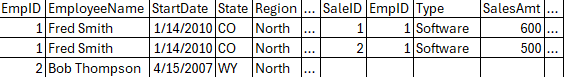
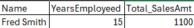
We are almost done with the clauses as we come up to Phase 8: the DISTINCT clause. In our example we do not have a DISTINCT clause, but this is where you can remove duplicates based on all fields in your SELECT clause. So if you had something like below from Phase 7, where there were two Jane Doe’s, both started the same year and both had the same total sales amount:
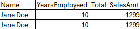
If we had a distinct on this, then it would return only one row:

As an important aside here: Do not use DISTINCT as a quick fix to remove duplicates. If you do not expect duplicates, then investigate why. There may be something wrong with your joins to cause a bit of a cartesian join somewhere which is duplicating rows by mistake. Distinct is very resource intensive, especially if you have a ton of rows you have to look at to see if there are duplicates. You are much better off fixing the query if it’s causing the duplicates.
Phase 9: ORDER BY – Sorting the Results
We move back down to the bottom of the query in Phase 9 with the ORDER BY clause. SQL Server does not ever guarantee the order of your results. Even if you are running a simple SELECT * from dbo.Sometable where that Sometable has a clustered index. The only way to guarantee your results are in a specific order is to use an ORDER BY clause.
(7) SELECT TOP 50 e.EmployeeName Name, DATEDIFF(Year, e.StartDate, GETDATE()) YearsEmployed, SUM(s.SalesAmt) Total_SalesAmt
(1) FROM dbo.EmpTable e
(2) LEFT JOIN dbo.SalesTable s
(3) ON e.EmpID = S.EmpID
AND s.Type = ‘Software’
(4) WHERE e.Region = ‘North’
(5) GROUP BY e.EmployeeName, DATEDIFF(Year, e.StartDate, GETDATE())
(6) HAVING SUM(s.SalesAmt) >= 1000
(9) ORDER BY YearsEmployed DESC, SUM(s.SalesAmt) DESC, e.EmployeeName
As you can see above, you can use the alias (YearsEmployed) or you can use the actual calculation (SUM(s.SalesAmt)), or the real field name even if it’s aliased (e.EmployeeName). In fact, you could even use the ordinal value of the field in your select statement if you wanted (eg, ORDER BY 2). WARNING: Anyone having to review your query is likely going to be cursing your name in the future! Plus, if you change the order of your SELECT clause in the future, you will need to remember to change the ordinal value, as well.
Phase 10: TOP – Limiting the Final Rows
FInally, we are at the last one, Phase 10 — the TOP clause. This is what will limit your query results to a maximum number of records. You can even add the keyword PERCENT after the number to get the top x-percent of the results (eg, TOP 10 PERCENT). If you have the result set ordered, like we do in this query, you’ll get that TOP x-number/percent back in that same order. If you did not use an ORDER BY clause, then you will just get the first x-number/percent records back.
(7 and 10) SELECT TOP 50 e.EmployeeName Name, DATEDIFF(Year, e.StartDate, GETDATE()) YearsEmployed, SUM(s.SalesAmt) Total_SalesAmt
(1) FROM dbo.EmpTable e
(2) LEFT JOIN dbo.SalesTable s
(3) ON e.EmpID = S.EmpID
AND s.Type = ‘Software’
(4) WHERE e.Region = ‘North’
(5) GROUP BY e.EmployeeName, DATEDIFF(Year, e.StartDate, GETDATE())
(6) HAVING SUM(s.SalesAmt) >= 1000
(9) ORDER BY YearsEmployed DESC, SUM(s.SalesAmt) DESC, e.EmployeeName
Logical vs. Physical Processing: What’s Next?
Remember, this is just how SQL Server will logically process this query; this is not how it will physically process it. That will be determined by the query optimizer and will involve any number of operators depending on how SQL Server thinks it will best be able to get you the data.
SELECT (Transact-SQL) – Microsoft Learn If you want to read the official word from the source, the Microsoft documentation for the SELECT statement covers this logical processing order in detail.
Itzik Ben-Gan’s Simple Talk Articles As I mentioned, Itzik Ben-Gan’s books were a huge help for me. You can find more of his articles and resources over at his Simple Talk author page.
Before reading this, did you realize that SELECT happens so late in the process (Phase 7)? How does this change how you view your aliases?